Chapter 2 was all about numerical linear algebra where we learnt the techniques of solving linear system of equations using both direct and iterative methods. Chapter 3 is all about finite difference approximation of derivatives which commonly arise in many daily life. We looked into forward, backward and central difference approximation of the derivatives. The forward and backward difference methods are $O(\Delta x)$ while central difference approximation is $O(\Delta x^2)$. For better accuracy of approximation, I would recommend to use the central difference method.
Integration is the process of measuring the area under a function plotted on a graph. The question one would like to know is Why would we want to integrate a function? Among the most common examples are finding the velocity of a body from an acceleration function, and displacement of a body from a velocity function.
Numerical integration is also an important technique. We started off with the simplest method called "Trapezoidal rule" which approximates the integral $I= \int_a^b f(x) dx $ where $a$ and $b$ are lower and upper bounds of the integral through a polynomial of order 1 i.e a linear approximation. The Simpson's $\frac{1}{3}$ rule and $\frac{3}{8}$ rule approximates using a quadratic and cubic polynomial. The main disadvantage of $\frac{1}{3}$ rule is that the number of intervals (n) should always be "even". If "n" is not even, I would either use Trapezoidal rule or Simpson's $\frac{3}{8}$ rule. Trapezoidal and Simpson's rule are all part of Newton-Cotes integration formulas. We shall also talk about "Two-point Gauss Quadrature rule" which is an extension of "Trapezoidal rule" where the arguments of the function are not predetermined as $a$ and $b$ , but as unknowns $x_1$ and $x_2$
$$I= \int_a^b f(x) dx=c_1 f(x_1)+c_2 f(x_2)$$
We shall derive the formula in the lecture on Friday
Thursday, February 11, 2010
Wednesday, January 20, 2010
LU Decomposition Vs Gaussian Elimination
In my last two lectures, I talked about Gaussian elimination and LU decomposition methods to solve a linear system of equations. I should have emphasized that while performing the row reduction operations, one can switch the rows as well.
The LU decomposition looks more complicated than Gaussian elimination. Do we use LU decomposition because it is computationally more efficient than Gaussian elimination to solve a set of n equations given by [A][X]=[B]?. For a square matrix [A] of $n \times n$ size, the computational time $CT_{DE}$ to decompose the [A]matrix to [L][U]form is given by
$CT_{DE}=T \bigg( \frac{8n^3}{3}+4n^2-\frac{20n}{3}\bigg)$, where $T=clock cycle time^2$.
The computational time $CT_{FS}$ to solve by forward substitution [L][Z]=[B] is given by$CT_{FS}=T(4n^2-4n)$The computational time $CT_{BS}$ to solve by backward
substitution [U][X]=[Z] is given by $CT_{BS}=T(4n^2+12n)$
The total computational time required to solve by LU decomposition is given by
$CT_{LU}=CT_{DE}+CT_{FS}+CT_{BS}$
$ = T \bigg( \frac{8n^3}{3}+4n^2-\frac{20n}{3}\bigg)+T(4n^2-4n)+T(4n^2+12n)$
$ = T\bigg( \frac{8n^3}{3}+12 n^2+\frac{4n}{3} \bigg)$
If we now consider Gaussian elimination the computational time taken by Gaussian elimination. The computational time $CT_{FE}$ for the forward elimination part is given by
$CT_{FE}= T \bigg( \frac{8n^3}{3}+8n^2-\frac{32n}{3}\bigg)$
The computational time $CT_{BS}$required is $T(4n^2+12n)$ and the total computational time is given by $ CT_{GE}= CT_{FE}+CT_{BS}= T\bigg( \frac{8n^3}{3}+12 n^2+\frac{4n}{3} \bigg)$ which is the same as LU decomposition.
This part of analysis leads to a confusion whether to use Gaussian elimination or LU decomposition. Let us now look at finding the inverse of a matrix. If we consider a $n \times n $ matrix. For calculations of each column of the inverse of the [A] matrix, the coefficient matrix [A] matrix in the set of equation [A][X]=[B] does not change. So if we use the LU decomposition method, the [A]= [L][U] decomposition needs to be done only once, the forward substitution (Equation 1) n times, and the back substitution (Equation 2) n times.
$CT_{INv LU} =1 \times CT_{LU} +n \times CT_{FS}+n \times CT_{BS}$
$ = T\bigg ( \frac{32n^3}{3}+12n^2-\frac{20n}{3}\bigg)$
In comparison, if Gaussian elimination method was used to find the inverse of a matrix, the forward elimination as well as the back substitution will have to be done n times. The total computational time $CT_{INv GE}$ required to find an inverse of a matrix is given by
$CT_{INv GE}= n \times CT_{FE}+n \times CT_{BS}$
$ = T\bigg( \frac{8n^4}{3}+12 n^3+\frac{4n^2}{3}\bigg)$
Clearly for large $n$, $CT_{INv GE} >> CT{INv LU}$ as $CT_{INv GE}$ has a dominating $n^4$ term where as $CT_{INv LU}$ has a $n^3$ term.
Sunday, January 17, 2010
End of root finding techniques
I am now done with root finding techniques. The sections covered so far are
• Types of errors in numerical computation (1.8) (0.4-0.5)
• Root finding methods for nonlinear equations (8.1-8.2) (1.1-1.6).
I will be posting some review questions as I go along with the lectures. I also strongly encourage to try out the programs provided in the textbook by Grasselli \& Pelinovsky to get more exposure to the techniques I discussed in my lectures. Try the program which solves for multiple roots using Newton's method and see whether you can get quadratic convergence!.
Wednesday, January 13, 2010
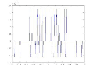
Zero Plot
The plot of zero should like this. The upper bound of the value is fixed to $O(10^{-16})$
%%%%%%%%%%%%%%%%%%%%%%%%%%%%%%%%%%%%%%%%%%%%%%%%%%%%%%%%%%%%%%%%%%%%%%%%%%%%%%%%%%%%%%%%
The below small program shows to draw a contour plot of the function I used
x=[-3:0.1:3];
y=x;
[X Y]=meshgrid(x,y)
contour(X, Y, X.^2+Y.^2,[4 4])
hold on;
contour(X,Y,exp(X)+Y,[1 1])
grid on;
%%%%%%%%%%%%%%%%%%%%%%%%%%%%%%%%%%%%%%%%%%%%%%%%%
$x^2+y^2=4, \quad e^x+y=1 $. Type this command in Matlab
If you need to solve the above equation
>> [X Y]=solve('x^2+y^2=4','exp(x)+y=1')
and you should obtain
X =
-1.8162640688251505742443123715859
Y =
0.8373677998912477276581914454592
Tuesday, January 12, 2010
3rd Lecture-Newton's method in 2 variables
I talked about fixed point method for finding a root of a non-linear equation and also applying Newton's method to functions of two variables. Again because of the time constraint, I was unable to show the programs in the lecture. I will be definately doing that in my lecture on Wednesday. See you all there!
Friday, January 8, 2010
2nd lecture-Secant and Newton's Method
I explained Secant and Newton's method today in the lecture and demonstrated with an example $f(x)=3x+\sin(x)-e^x$. I shall demonstrate the working code in my lecture on Monday. I should have written the general expression for Secant's method as
$$ x_{n+2}=x_n-f(x_n)*\frac{x_{n-1}-x_n}{f(x_{n-1})-f(x_n)}$$
where $n=1,2,3 \cdots$. Have a great weekend and see you all on Monday
$$ x_{n+2}=x_n-f(x_n)*\frac{x_{n-1}-x_n}{f(x_{n-1})-f(x_n)}$$
where $n=1,2,3 \cdots$. Have a great weekend and see you all on Monday
Wednesday, January 6, 2010
1st lecture
Hello folks,
Today was the 1st lecture to this course. I hope it was fun!. I talked about different errors one can come across while doing numerical calculations which was from Introduction & Review part from the course outline. I also went on talking about root finding methods for non-linear equations and started with bisection method and demonstrated a working code . I should have emphasized that this method works only when the criterion is satisfied and also this method is only for single root. I shall be talking about Secant, Newtons and Fixed Point methods on Friday. See you there!
Today was the 1st lecture to this course. I hope it was fun!. I talked about different errors one can come across while doing numerical calculations which was from Introduction & Review part from the course outline. I also went on talking about root finding methods for non-linear equations and started with bisection method and demonstrated a working code . I should have emphasized that this method works only when the criterion is satisfied and also this method is only for single root. I shall be talking about Secant, Newtons and Fixed Point methods on Friday. See you there!
Subscribe to:
Comments (Atom)